Continuum Electrostatics Calculations

Dr. Udo W. Schmitt, Max-Planck Institut fuer Biophysikalische Chemie, Goettingen

In the previous lecture we've learned about the importance of long-range electrostatic interactions for an accurate modeling of biomolecular macromolecules in aqueous solution. Today's practical will deal with the computation of these interactions by means of the so-called non-linear Poisson-Boltzmann equation (PBE)

introduced during the last lecture.

In the equation above is the number density of ions of type i in the bulk solution,

is the charge on the ion, is the electrostatic potential in that region of space, is Boltzmann's constant and is the temperature.

is the charge density due to the macromolecule under consideration. Note that the dielectric constant epsilon(x,y,z) is a function of the location in R3 (inhomogenous epsilon). The nonlinear PBE given above can be linearized

via a Taylor expansion of the sum at the right hand side (as being shown last week).

To obtain solutions of the PBE on a computer, we are going to use APBS (Adaptive Poisson-Boltzmann Solver), a software package for evaluating the electrostatic properties of nanoscale biomolecular systems, which is already installed on the computers you are working with. APBS

solves the Poisson-Boltzmann equation numerically by means of a finite difference/finite element

approach. For more details on this, please see the official program web site.

The files needed for this practical can be downloaded here. You will need to unpack

the archive by typing:

tar xzvf PBE_prakt.tar.gz

Simple example: Born solvation

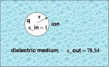
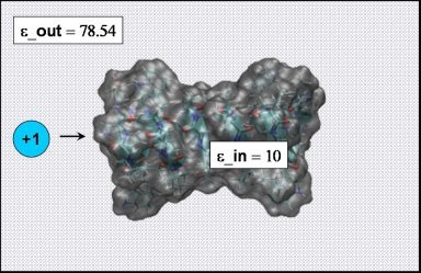
As a first and rather straightforward step we are computing the solvation free energy of a ion with charge q and radius a (or r in the picture to the right) embedded in a dielectric continuum with dielectric constants epsilon_out. The ion itself has a dielectric constant of epsilon_in. In other words, epsilon_in and epsilon_out denotes the internal and external (solution) dielectric constants, respectively. If epsilon_in is chosen to be 1, the result obtained is the free energy change associated with transfering an ion from the gas phase into a solute with dielectric constant epsilon_out.

In our Born solvation model we assume zero ionic strength.

Two things are needed to run a calculation with APBS:

an input file for APBS and

a so-called PQR file, which is an augmented PDB file that also contains the partial charge and the radius of the respective atom in the occupancy and temperature columns, respectively.

For our Born solvation model the PQR file only contains one atom with partial charge +1.

It looks like this:

REMARK This is an ion with a 3 A radius and a +1 e charge

REMARK located at position (0.,0.,0.)

ATOM 1 I ION 1 0.000 0.000 0.000 1.00 3.00

The input file for APBS is somewhat more extended and looks like this:

# READ IN MOLECULES

read

mol pqr born.pqr # Read molecule 1

end

# CALCULATE POTENTIAL FOR SOLVATED STATE

elec name solvated

mg-manual

dime 65 65 65

nlev 4

grid 0.33 0.33 0.33

gcent mol 1

mol 1

lpbe

bcfl mdh

pdie 1.0 # Solute dielectric

sdie 78.54 # Solvent dielectric

chgm spl2

srfm mol

srad 1.4

swin 0.3

sdens 10.0

temp 298.15

gamma 0.105

calcenergy total

calcforce no

write pot dx pot

end

# CALCULATE POTENTIAL FOR REFERENCE STATE

elec name reference

mg-manual

dime 65 65 65

nlev 4

grid 0.33 0.33 0.33

gcent mol 1

mol 1

lpbe

bcfl mdh

pdie 1.0

sdie 1.0 # Solvent dielectric

chgm spl2

srfm mol

srad 1.4

swin 0.3

sdens 10.0

temp 298.15

gamma 0.105

calcenergy total

calcforce no

end

# COMBINE TO FORM SOLVATION ENERGY

print energy solvated - reference

end

# SO LONG

quit

First, APBS reads the PQR file named born.pqr. Then two PBE calculations with different solvent dielectric constant, 1 and 78.54 (why are we using this value?), respectively, will be performed (named solvated and reference), and the difference between these two free energies will be printed at the end of the run (Please note: you do not need to know the precise meaning all the other parameter in the APBS input !!!)

Compare your computed result with the analytical value obtained via

where R is the radius of the ion. Where does the small error come from?

You can change the radius in the PQR file, repeat the calculation and compare

again the numerical and the analytical result.

We can now also display the electrostatic potential by typing

vmd -e pot_field.vmd

Electrostatic potential of the ion channel Gramicidin A

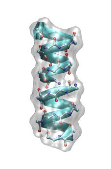
Now we are ready to perform a PBE calculation on a biomolecular macromolecule. To this end we have chosen

the ion channel Gramicidin A (gA) in its helical form. Gramicidin A is a derivative of gramicidin, an

antibiotics consisting of a heterogeneous mixture of six antibiotic compounds. Gramicidin A is a linear polypeptide containing 15 amino acids. It kills pathogenic organisms by destroying the cationic (Na+,K+,H+) concentration gradients that are vital for their proper functioning. In other words, monovalent cations

can easily leak through gA once it got incorporated into the cell membrane of the organism.

Have a look at the structure of helical gA dimer by typing

vmd -e gA.vmd

and rotating the polypeptide.

Also have a look at the SYSTEM.pqr file. What is so far the (only) major difference compared to the previous Born ion example?

At this point we need to specify the internal (i.e. inside the protein) dielectric constant for our calculation

(remember: in the Born solvation case the internal dielectric constant was set to 1).

With the dielectric constant being a macroscopic observable, but the biomolecular macromolecule

being a nano-sized molecular entity, it is often not clear what value

to choose, and one should consider the internal dielectric constant as an adjustable parameter within the PBE framework. It usually ranges from 2 to 20, depending on the molecular details of the macromolecule under consideration. (What determines the lower bound of the range?)

We can now easily perform the PBE calculation inside VMD. VMD - Visual Molecular Dynamics - is a molecular visualization program for displaying, animating, and analyzing large biomolecular systems using 3-D graphics and built-in scripting. You need to highlight the "START.pdb"

representation in the "Main" window, right mouse click and choose "Load data into molecule". Then

chose "SYSTEM.pqr" and type "Load". This will load the PQR file for gA.

Now go to the "Extensions" section in the "VMD Main" window and select "Analysis -> APBS Electrostatics". Click on "Edit" and change the number of the x,y,z grid points from 129 to 65. Also change the

solute (protein) dielectric constant to 10. Start the PBE calculation by pressing "Run APBS".

You can follow the APBS computation in the "vmd console" window. After completion accept to load the electrostatic potential into the top molecule. Now add two new graphical representation "Isosurface" via "Graphics - > Representation", one for the negative part and another one for the positive values of the potential. Change the values

of the isocontours and look what is happening to the molecular representations.

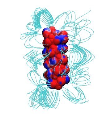
One can also map the electrostatic potential onto a generated molecular surface. For example one can

compute the so-called solvent-accessible surface by rolling a contact sphere with a given radius over the

macromolecule and then grouping (triangulating) all sphere center points into one surface. To do this, we delete the two isosurface representations from the previous example. Add a new representation "Surf" and change the probe radius to 1.1 Angstroem. Then change the "Coloring method" to "Volume" and in "Trajectory"

adjust the "Color Scale Data Range" to -1 and 1, respectively.

Now you can zoom into the channel region. The striking feature is that the channel area as well as the entrance area show the same coloring, which means the sign of the potential is the same. What sign of

the potential whould you expect for a cation selective channel?

We can check on the sign of the potential by inspecting the coloring scheme used in the representation.

To do so we go to "Graphics -> Color - Color Scale".

Ion permetation free energy profile for Gramicidin A

In order to compute the free energy profile for cation migration through gA using the PBE

we only need to add one cation to an existing PQR file of gA and repeat the calculations from the previous

example for varying ion positions. To speed up the process, there are already 9 PQR files with equidistant ion positions spanning the range from -16.0 to +16.0 Angstroem in your working directory. Please have a look at one of the SYSTEM.pqr.* files

first.

ATOM 547 HA2 ETA 17 2.016 -10.455 -4.104 0.090 1.320

ATOM 548 CB ETA 17 2.566 -12.311 -5.091 0.050 2.175

ATOM 549 HB1 ETA 17 2.983 -13.305 -4.818 0.090 1.320

ATOM 550 HB2 ETA 17 1.624 -12.457 -5.663 0.090 1.320

ATOM 551 OG ETA 17 3.493 -11.626 -5.922 -0.660 1.770

ATOM 552 HG1 ETA 17 3.762 -12.236 -6.614 0.430 0.224

ATOM 553 Na ION 3 -2.675 16.000 -1.764 1.000 1.908

END

We can also have a look at the sequence of differing ion positions inside gA by typing

vmd -e snapshots.vmd

As in the Born solvation example, we also need to compute a reference state that only

contains the cation embedded in pure water ( those coordinates can be found in the ion.pqr.* files: have a look at one of them).

If we substract the two computed free energies we get the difference in free energy

between the cation being solvated by pure water and the cation being solvated at a fixed position by gA, which is hydrated by water (Note that we are only interested in the free energy difference, so no complete thermodynamic cycle needs to be computed!). The working directory contains a script that will

perform the 9 independend pairs of PBE calculations and write the total free energy into a file

named "total_energy". The APBS parameters are given in apbs.in (What solute dielectric constant

is initially used?).

You can now start the script by typing

./PBE_loop

For each snapshot shown the script will run a PBE calculation and extract the solvation free energy difference (you will have to eventually merge it into the respective cation position).

After the calculation is finished, you can plot the free energy profile using e.g. "gnuplot"

gnuplot

plot "total_energy" w lp

plot "total_energy" u :1 smooth csplines w lp

Why should the profile be symmetric? Why is it not the case?

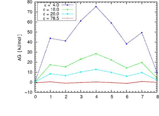
You can now change the solute dielectric constant in the "apbs.in" file, repeat the previous

computation cycle and eventually try to reproduce the plot shown below (in case there is time left).

The graph illustrates the dependence of the free energy profile

as a function of the protein dielectric constant. The free energy barrier for Na+ migration

through gA is estimated to be ~ 50 kJ/mol. Which dielectric constant will give a result close to

experiment? Which dielectric constant would you choose if there would be no experimental value

to compare with?

What can we learn from this plot? Does it have the right asymtotics as epsilon_in -> 78.54?