Rate theory@work

Dr. Udo W. Schmitt, Max-Planck Institut für Biophysikalische Chemie, Göttingen
In the previous lecture we've learned about the theoretical basis of chemical reaction rate theory. In particular, we looked at Transition State Theory (TST) (or the theory of the activated complex) and Kramers Theory (KT).
In this practical we are going to investigate in detail on these two theories.
To this end, we will compute molecular dynamics trajectories using the so-called Langevin equation,

which basically describes Newtonian dynamics with an additional friction term
with a time-independent friction constant plus a random force that ensures proper thermalization of our system.
The random force R(t) is Gaussian white noise with zero mean and obeys the fluctuation-dissipation relation. Note that the Langevin equation also provides the fundamental basis in Kramers Theory (see previous lecture).
All calculations performed in this practical will be done with a simple molecular dynamics
program written in Fortran 77/90 that solves the Langevin equation for single degree of freedom x (i.e. one particle) in a symmetric double minimum potential. In case you are interested in the details you can have a look at the source code langevin.f. To compute the rate after we have generated a trajectory we use a short analyzing program
called rate.f.
To start the practical download the relevant files from here followed by unpacking them with the following command
tar xzvf rate_prakt.tar.gz
Then change into the new directory and compile both programs needed with
gfortran langevin.f -o langevin

gfortran rate.f -o rate
Now we are ready to run our first computation. Our first task will be to have a look
at the potential V(x) that will govern the deterministic part of our Langevin dynamics.
To plot the potential V(x) just start the program langevin by typing
./langevin md.in
and then start a Linux plot program, like for example gnuplot
gnuplot (RETURN)

p "POTENTIAL" u 1:2 w l

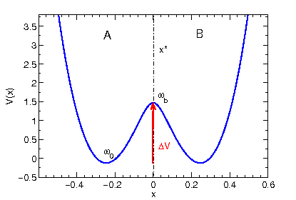
(A symmetric double minimum potential should appear on the screen.)
The potential is a generic example for all kinds of reactive processes
that show no potential (or free energy) difference between the two
metastable regions A and B. The dynamical variable x is our order parameter
(or reaction coordinate, collective variable or meta-coordinate) that must be able
to distinguish between region A and B. Thinking in terms of macromolecules
it would be a collective coordinate like e.g. the number of native contacts,
the solvent-accesible surface of the radius of gyration. You can also view
it as a projection from 3N cartesian coordinates of your macromolecule
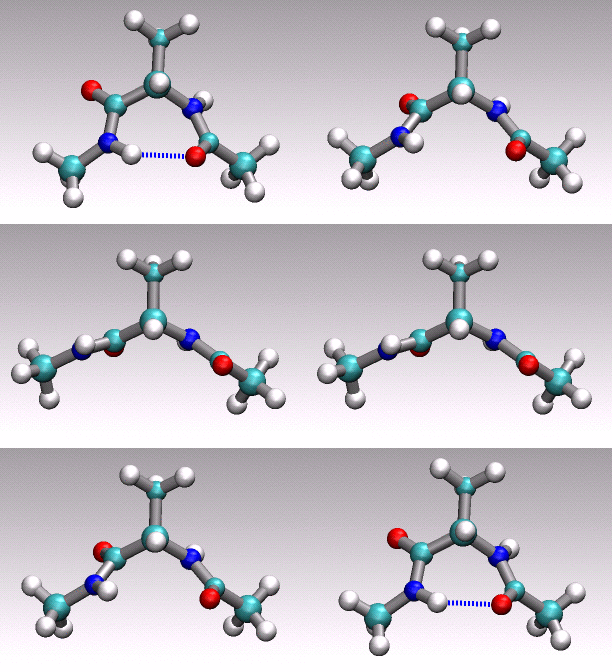
at hand onto a 1D (collective) coordinate. For example in the animation of
a distinct conformational transition in alanine dipeptide shown above one could
imagine to use an angle or a hydrogen-bond distance as order parameter
to arrive at a reduced 1D description of the overall reactive process
describe by the concerted movement of all 22 atoms shown.
The input file md.in of our MD program contains the necessary parameters shown here
4000  1       # nsteps,nout

0.005         # timestep

0.2           # x(t=0)

0.0           # temperature

0.0           # friction coefficient

.F.           # compute TST and Kramers rate
that will be read by the program langevin prior to the computation.
The parameters will be explained briefly in the following: nsteps are the total
number of molecular dynamics steps performed, nout gives the inverse
output frequency (ouptut is written only every n'th step), timestep is the discrete
time step used in the numerical integration algorithm, x(t=0) are rather self-explanatory, temperature is the reduced temperature and friction coefficient is the parameter gamma that enters the Langevin equation. Note that the program uses a reduced unit system with k_B = 1, i.e. the temperature is given
in units of energy.
Now we can start our first simulation with the input parameters and look at the resulting trajectory. Typing
./langevin md.in
there should now be a file TRAJECTORY
in your directory. We can display the content of this file by starting gnuplot and typing
p "TRAJECTORY" u 1:2 w l
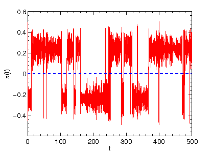
This should reveal the time evolution (time on the x axis) of the coordinate x (shown on the y axis) that evolves in double minimum potential according to Newton's equation of motion (Note that the friction coefficient and temperature in the input file are both zero).
The signal we obtain with the previous input setting is representative of so-called ballistic dynamics (as opposed to diffusive dynamics we will
encouter later on). The particle oscillates between the two potential wells
with constant total energy (try in gnuplot p "TRAJECTORY" u 1:4 w l,"TRAJECTORY" u 1:5 w l to display the time evolution of the potential energy and total energy).
What is the rate k
for a process like this?
Now we can turn on the friction term by setting gamma in the md.in input file
to a finite value (e.g. 0.5) and starting the previous simulation with otherwise identical parameters. What behaviour do you see now? What is the difference to the previous example?
Try to run a trajectory with the initial coordinate x located at the barrier top and try to explain the observed behaviour.
Finally we are going to also turn on the random force (see Langevin equation) in order
to counteract the damping that is introduced by the friction term. What different physical mechanism are mimiced by the friction term in connection with the random force?
By setting temperature to 0.75 and starting the simulation again we obtain now a different time evolution of x. How many reactive event (crossing from A to B) do you observe for this short trajectory? Again try to run a trajectory with the initial coordinate x located at the barrier top and try to explain the observed behaviour. What is different compared to the previous example with R(t) = 0?
Being done with the preliminaries we can begin with computing reaction rates from our trajectories. To do so, we have to increase the number of integration steps nsteps
in md.in such that we observe a sufficiently large number of reactive events.
To compute the rate from our trajectory, we run a second program rate that reads
in TRAJECTORY file and performs a smart counting of reactive events, i.e. how often
does a the dynamical variable x move from region A to region B. We simply start
the program by typing
./rate
and it will give us the rate k which has dimension 1/(time) and units 1/(timestep), where
timestep is the specified timestep in md.in
Next we are going to analyze whether our simple 1D model shows the expected Arrhenius behaviour. In the previous lecture we learned that the reaction rate as a function of temperature follows a phenomenological law (Equation), which means that a plot ln(rate) vs. 1/T should reveal a straight line. To check this result we perform rate computations at four different temperatures (0.25 0.5 0.75 1.0) and from each extract the rate k and plot the combined data in gnuplot
p "arrhenius.dat" (1./$1):(log($2)) w lp

