Combining Molecular Dynamics with Electronic Structure Calculations methods
Dr. Udo W. Schmitt, Max-Planck Institute for Biophysical Chemistry, Goettingen
In the previous lecture we've learned about Density Functional Theory-based electronic structure
methods as a viable alternative to the Hartree-Fock approach.
Today we are going to combine the already introduced molecular dynamics (MD) approach with
two electronic structure methods, which will lead us to the field of
so-called ab initio molecular dynamics or "on the fly" (direct) MD. This is opposed to
the common force field techniques that are used to represent the potential energy surface,
where the potential energy (and thus the forces on the nuclei) are determined
before we start our simulation. In ab initio dynamics the forces are computed "on the fly", i.e.,
at every new set of coordinates generated during our molecular dynamics run. To this end,
for every new set of coordinates an independent electronic structure calculation needs to be
performed in order to compute the interaction energy and the forces on the atoms (nuclei).
The package we going to use for the electronic structure computation is again MOLPRO (see previous practical), which has been developed
by Peter Knowles and Hans-Juergen Werner over the last 15 years. MOLPRO has been used in the previous
practical as well.
In order to be able to perform "on the fly" dynamics, we also need a MD program that acts as a driver
for the electronic structure calculation. Here we going to use speedEVB, which is a molecular
dynamics packages that provides a numerically efficient implementation of the Multistate
Empirical Valence Bond (MSEVB) model together with a combined direct dynamics/QM/MM interface.
The term QM/MM stands for Quantum Mechanics/Molecular Mechanics and was together with the MSEVB
model introduced in the previous lecture .
The files needed for this practical can be downloaded here. You will need to unpack
the archive by typing:
tar xzvf prakt2.tar.gz

ulimit -s unlimited
Direct Molecular Dynamics using the Multistate Empirical Valence Bond (MSEVB) model
In this ection we are going to perform MD calculations on proton transfer through
a so-called water wire. To be able to do so, we need a model of our potential energy surface that allows
for explicitly break and form chemical bond. A model that allows for that in an elegant way
is the Multistate Empirical Valence Bond (MSEVB) to describe the reactive potential energy surface (PES). The MSEVB model (also see previous
Lecture) provides a simple and numerical efficient way of modeling chemical reaction
dynamics in aqueous systems. The MSEVB approach is nowadays used extensively in biomolecular
simulations to study proton transport phenomena in molecular detail.
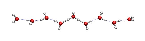
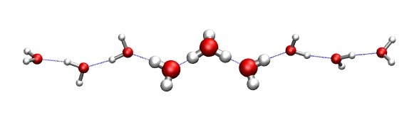
A water wire is a onedimensional alignment of water molecules that
are held together via hydrogen bonds. In case the water molecules are aligned properly, a
proton can migrate through the water wire by the so-called Grotthus mechanism. Grotthus
mechanism means that though a proton is transfered from one end to the other of the wire,
the movment of the individual atoms is quite small, i.e., a few tenth of an Angstroem.
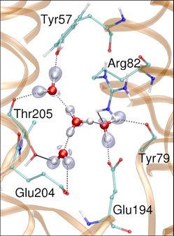
Aligned water wires are found in a variety of proteins, like e.g. in Bacteriorhodopsin or
Cytochrome c Oxidase, where they constitute a crucial part of the proteins functionality.
That means that lack of the water wire will lead to misfunction of the respective protein.
In this course we are going to focus on the water wire plus one excess proton only and are mimicking
the protein via a cylindrical trapping potential that will keep the water molecules aligned in
single file.
First have a look at the starting structure located in the directory sim/ by typing
vmd start.pdb
and locate the water molecule that carries the excess proton.
Now we are going to perform a MSEVB molecular dynamics simulation with this starting structure
speedEVB wire.in
The program will report all its events to the screen output and will finish after 1000 MD steps.
You can have a look at the generated trajectory by starting the VMD script:
vmd -e wire.vmd
Locate the excess proton and following its dynamical path through the water wire. How many bonds are formed and broken along the pathway?
Besides the trajectory additional information has also been written
to the file system. Have a look at the energies, i.e., kinetic energy, potential energy and total energy, by
typing
gnuplot kin_energy.gplot

gnuplot pot_energy.gplot

gnuplot energy.gplot
What do you expect for the total energy of a system that follows Newton's (or Hamilton's) equation of motion?
In the directory transfer/ you can start a shorter simulation run by typing
speedEVB wire.in
Now you can have a look at the amplitudes of the individual ground state electronic expansion coefficients for the localized valence bond states as a function of simulation time. The amplitudes
give you the fraction of the total charge of +1 (the proton charge)
that resides on each water molecule at a given time. Typing will display the results:
gnuplot evb_amplitudes.gplot
How does the time evolution of the electronic expansion coefficients reflect the proton transfer events
seen in the previous VMD movie?
VMD also allows you to visualizes the electronic expansion coefficients as changing color/size
on the individual water molecules. Simply type
vmd -e amplitudes.vmd
Identify on how many water molecules the excess charge is distributed at a given time. Can the
transfer process be described in a picture where the excess charge of +1 is localized on a single
water molecule?
Direct Molecular Dynamics using Density Functional Theory in Combination with a QM/MM ansatz
With the same system as in the previous example - a protonated water wire - we are now going to
perform mixed quantum-classical (QM/MM) molecular dynamics simulation. The first thing we have
to define is the extend of the QM region, i.e., the part of the total system that is treated
by means of an electronic structure method. The rest of our system will be handled by standard force
field. The QM region will be the core region of our protonated water cluster that is embbeded
in the overall water wire and is simply defined in the input files (fort.10) as:
QM_REGION

  10

  1 2 3 4 5 6 7 8 9 10
That just means that the first ten atoms will be treated as quantum-mechanically (QM_REGION), and the rest will be considered as being part of the MM treatment. See the picture to the right that shows the QM (H7O3+) cluster in thick ball-and-stick representation.
For the QM computation, which will be performed with MOLPRO, we will have to specify the electronic structure method that will be used (Hartree-Fock, Density Functional Theory, Moeller-Plesset etc.)
and an appropriate basis set. This is done in the input file "qm.com":
basis=midi

geomtyp=xyz

GEOMETRY=qm.xyz

set,charge=+1

ks,b3lyp
Compare to last weeks practical only the command "ks, b3lyp" (which stands for Kohn-Sham) appears as the new DFT key word, and "b3lyp" specifies the density functional that is used during the calculation.
To start our simulation, which will perform 40 molecular dynamics steps, just type
speedEVB_qmmm wire.in
You can follow the
screen output: this calculation will take a couple of minutes.
After successful finish you can look at the generated trajectory by typing
vmd -e wire_qm.vmd
QM/MM Molecular Dynamics of Protonated Water Clusters in Bacteriorhodopsin
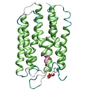
Our last task for this semester will be to compute a short trajectory using the technqiues
introduced above on a model of the light-driven proton pump Bacteriorhodopsin. Bacteriorhodopsin
absorbes light in the visible range and converts this energy via a cascade of proton transfer
steps into chemical energy. It can be regarded as a simple model system for larger protein complexes
that perform light-driven energy conversion, like for example the Photosynthetic Reaction Center that is found in
plants.
All necessary input files are given in the working directory "bR_QMMM", so you only need to type
speedEVB_qmmm bR.in
to start the simulation. In total 20 steps will be performed and can be displayed using VMD
vmd -e bR.vmd
Shown are the protein in a so-called "Ribbon" representation that highlights secondary structure
elements and the QM region consisting of 3 water molecules and one excess proton at the extracellular entrance area of Bacteriorhodopsin.
tail -100 fort.10
will show you the simple definition of QM atoms. Note that we could select any region within the
molecule to be treated at the high-level of theory - Hartree-Fock or Density Functional Theory -
in order to compute observables with high accuracy.