Introduction to Electronic Structure Calculations using MOLPRO
Dr. Udo W. Schmitt, Max-Planck Institut fuer Biophysikalische Chemie,Goettingen
In the previous lecture we've learned about the theoretical basis of electronic
structure methods, and in particular about the Hartree-Fock method.
Now it is time to jump into the electronic structure business and perform
a couple of calculations by yourself.
The package we are going to use is called MOLPRO, which has been developed
by Peter Knowles and Hans-Juergen Werner over the last 15 years. It is among
the modern electronic structure codes available and provides an easy-to-use scripting language that allows for
a user-friendly access to quantum chemistry. Additionaly MOLPRO provides for the largest set of implemented post-Hartree-Fock methods.
To learn how to use the program by yourself or maybe extend your knowledge beyond the
scope of this tutorial one can check out the
links "Quick Start" or "User's Manual" on the following site
To start a calculation we basically need four things:
- the structure of the molecule of interest in (cartesian) coordinates
- the overall charge of our system
- the method that will be used (Hartree-Fock (HF),
Density Functional Theory (DFT), Moeller-Plesset perturbation theory (MPx) etc.)
- a basis set.
The files needed for this practical can be downloaded as an archive here
and unpacked by typing
tar xzvf prakt1.tar.gz
The H-H molecule
Our first calculation will be the simple H2 molecule, which is the smallest
molecule that exhibits all fundamental aspects of chemical bonding (why?).
A simple input for the electronic structure calculation of H2 is given below:
basis=6-31G

r=1.0 ang

geometry={angstrom;

          h1;

          h2,h1,r}

hf
First, the basis (6-31G) using the so-called Pople notation is specified. G stands for "Gaussian", so a GTO basis with 6 gaussian functions for the inner (non-valence) electrons and 4 (3+1) for
the valence electrons is used. Then, the H-H distance and the so-called internal coordinates (bonds,angles, torsions) are specified.Finally, the key word "hf" stands for "do a Hartree-Fock calculation"
Now we start out first electronic structure calculation by typing
molpro h2.com
During the calculation MOLRPO writes an output file that communicates the most
important infos to the user. Please extract the following information:
- number of SCF cycles needed for convergence
- the HF energy (what units are being used?)
- the dipole moment
Additionaly you could extract the individual HF energies after each SCF cycle and plot them
against the number of cycles.
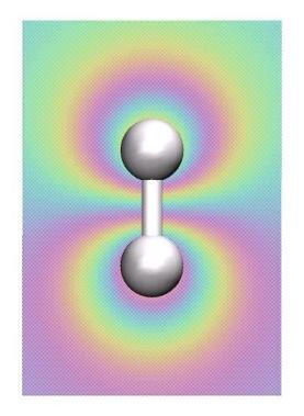
In the next step we want to perform the visualization of the bonding and antibonding molecular
orbitals (MO) of the H2 molecule. For this we have to redo are electronic structure calculation:
molpro h2_orbitals.com
The same calculation as in the previous step will be performed, but additionaly the MOs
and the electron density are written to external files. To view the MOs, we will have to use VMD, a molecular visualization program for displaying, animating, and analyzing large biomolecular systems using 3-D graphics and built-in scripting.
Typing
vmd -e orbitals.vmd
will load an existing script that loads the relevant MOs.
In the VMD main window you can activate(deactivate) the two MO and the electron density while clicking on the D entry for each MO/density entry in the main window. Which orbital is the bonding, which one is the anti-bonding one?
So far, we have only performed so-called single-point calculations, i.e. computed the HF energy
for a fixed nuclear configuration. MOLPRO is quite versatile when it comes to automatically
perform scans along selected coordinates. In our case of the H2, we will now
determine the energy profile (or the potential energy surface (PES)) along the H-H distance. The input
file now looks like this:
r=[0.3 0.4 0.6 0.8 1.0 1.2 1.4 1.6 2.0 4.0 6.0] ang

basis=6-31G

i=1

geometry={

          h1;

          h2,h1,r(i)}

do i=1,#r   !loop over range of bond distances

 hf

 e1(i)=energy

enddo

{table,r,e1

  title,HF PES for H-H

  plot,file='h2_hf_pes.plot'

}
the program will loop over all specified distances and perform for each of those an independent SCF calculation. Finally, a table of the respective HF energies will be written to a file called h2_hf_pes.plot
Now we going to use the plot program "xmgrace" that comes with most Linux distributions
to look at the PES. Typing
xmgrace h2_hf_pes.plot
will reveal the electronic HF energy as a function of the H-H distance.
What is the energy one would expect for the dissociation limit (i.e. r-> oo) of H-H?
As pointed out in the lecture, the HF method gives molecular interaction energies that are only
approximations to the exact quantum many-body energy. In the following we will study the effect
of improving the HF approximation. This will be achieved via perturbation theory, the so-called
Moeller-Plesset (MPx, where x gives the order in the perturbation expansion) and variational
multi-determinant methods, like e.g. configuration interaction (CI). In molpro this can simply be
achieved by adding the respective keywords:
r=[0.3 0.4 0.6 0.8 1.0 1.2 1.4 1.6 2.0 3.0 4.0 5.0 6.0] ang

basis=6-31G

i=1

geometry={

          h1;

          h2,h1,r(i)}

do i=1,#r   !loop over range of bond distances

 hf          ;e_hf(i)=energy

 mp2,NOCHECK ;e_mp2(i)=energy

 casscf      ;e_cas(i)=energy

 mrci        ;e_ci(i)=energy

enddo

{table,r,e_hf,e_mp2,e_cas,e_ci

  title,HF PES for H-H

  plot,file='h2_methods_pes.plot'

}
After a sucessful finish of the MOLPRO run you can have a look at the four PESs again using "xmgrace".
In our example the CI method (mrci) can be considered as the most accurate. CASSCF stands for "complete active space SCF", which can be regarded as a truncated CI expansion. Compare your result with respect to the obtained equilibrium bonding distance (How large is the error for this quantity?) and the dissociation limit for
each method. Hereby the CI results should serve as the reference energy curve. Repeat the calculation with changing the
order in the perturbation expansion from 2 to 4 (mp2 -> mp4) and compare the two results. What is the error in the CI result
compared to the analytical results of -1 Hartree. How can we improve the CI dissociation energy?
The water molecule
Now we going to move to a slightly more complex molecule having three nuclei and 10 electrons: the water monomer. For the structural information MOLPRO allows for the use of
the convient xyz in cartesian coordinates format. An example xyz-File is shown here:
    3

remark line

    O    0.00000   0.00000   0.00000

    H    0.00000   0.00000   0.94000

    H    0.00000   0.99030  -0.23192
With this structure, which does not represent the well-known equilibrium structure of water, we first have to perform a so-called geometry optimization. During the geometry optimization cycle a SCF calculation is performed. This one is used to compute the gradient of the total energy on the nuclei, which is then used
to perform a move of the nuclei. Then the new nuclei positions are feeded into a new SCF calculation. These
steps are repeated until the structure (=positions of the nuclei) does not change anymore.
The input file for a geometry optimization looks like this:
basis=6-31G                  !basis set

geomtyp=xyz

GEOMETRY=h2o.xyz

hf                           !Hartree-Fock

optg,savexyz=h2o_opt.xyz
Compare the optimized geometry "h2o_opt.xyz" with your input geometry "h2o.xyz" using VMD. Determine the bond distances and the bending angle in the water molecule. How does it compare to the experimental results? How can we further improve the structure? How many geometry optimization cycles were necessary to converge the geometry? (you could also plot the number of cycles against the corresponding HF energy using "xmgrace" or "gnuplot")
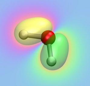
Using the optimized geometry, we are now computing the MOs of water.
Have a look at the input file "h2o_orbitals.com" first and try to analyze what is going on
in this type of calculation. Then type
molpro h2o_orbitals.com
The generated MOs can again be visualized using VMD:
vmd -e orbitals.vmd
Have a look at all occupied MOs and elucidate their role for bonding in the water monomer.
Which atomic orbitals of the individual atoms are predominately participating in each MO?
Compare the MOs with the ones shown on the following web site:
Molecular Orbitals of the Water Monomer
Caffeine
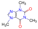
Finally we are gonna to compute the electronic structure of the well-known
Caffeine molecule, which is a xanthine alkaloid compound that acts as a stimulant in humans.
The structure of this biomolecule is shown to the left.
Type to start the HF caclulation:
molpro caffeine.com &

tail -f caffeine.out
and observe the information that is written to the screen.
How long does one SCF cycle take on average? How many electrons are involved during this computation?
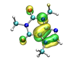
The so-called HOMO (highest occupied molecular orbital) can be visualized using VMD:
vmd -e orbitals.vmd
How many occpuied MO are there?
If there is some time left, try to compute all orbitals by changing "HOMO" to "ALL" in the input file.
Then visualize them along the same lines as in the previous example.