Protein structure determination by x-ray crystallography and NMR
In the last lectures we learned how protein structures are determined experimentally.
Today, we'll focus on how computational techniques are employed to aid
structure determination.
There are two main techniques for solving protein structures: x-ray
crystallography and Nuclear Magnetic Resonance (NMR).
As can be seen from the current
PDB holdings, more than 42,000 protein structures have been solved
so far, and are available from the
Protein Data Bank. About 13% of these are NMR structures, the rest
are x-ray crystallographic structures. As can also be seen on the PDB holdings list,
the number of solved proteins grows even faster, due to advancements
in structure determination techniques. Nevertheless, the number of
known protein sequences is almost an order of magnitude larger
(currently about 276,000, as available from the SWISS-PROT
database).
Reading PDB files
As we've learned last time, protein structures are stored at the Protein Data Bank, from which
individual protein structures can be retrieved as so-called PDB
files. Before we will turn to the structure determination itself, let
us have a closer look at a typical PDB file, to see what can be
learned about the background of the structure (experimental conditions
etc.) and the structural quality (the resolution, coordinate uncertainty).
We will focus on PDB entry 1TRO (an x-ray structure) as it can
be downloaded from the Protein Data bank.
The initial lines of a PDB entry contain information on the
protein, the source, the names of the people who sent the entry to the
PDB, references to literature that describe the structure in detail,
and some basic information regarding the crystallographic
data. Especially critical to check are the resolution and the R-factor
(or free-R factor), that contain information on how well the deposited
structure matches the measured data (x-ray reflection intensities in
this case).
HEADER    DNA-BINDING REGULATORY PROTEIN          30-AUG-92   1TRO      1TRO   2

COMPND    TRP REPRESSOR COMPLEX WITH OPERATOR                           1TRO   3

SOURCE    TRP REPRESSOR: (ESCHERICHIA COLI, STRAIN W3110);              1TRO   4

SOURCE   2 OPERATOR: SYNTHETIC                                          1TRO   5

AUTHOR    Z.OTWINOWSKI,R.G.ZHANG,P.B.SIGLER                             1TRO   6

REVDAT   1   31-JAN-94 1TRO    0                                        1TRO   7

REMARK   1                                                              1TRO   8

REMARK   1 REFERENCE 1                                                  1TRO   9

REMARK   1  AUTH   Z.OTWINOWSKI,R.W.SCHEVITZ,R.-G.ZHANG,C.L.LAWSON,     1TRO  10

REMARK   1  AUTH 2 A.J.JOACHIMIAK,R.MARMORSTEIN,B.F.LUISI,P.B.SIGLER    1TRO  11

REMARK   1  TITL   CRYSTAL STRUCTURE OF TRP REPRESSOR OPERATOR          1TRO  12

REMARK   1  TITL 2 COMPLEX AT ATOMIC RESOLUTION                         1TRO  13

REMARK   1  REF    NATURE                        V. 335   321 1988      1TRO  14

REMARK   1  REFN   ASTM NATUAS  UK ISSN 0028-0836                  006  1TRO  15

[..]

REMARK   2                                                              1TRO  23

REMARK   2 RESOLUTION. 1.9  ANGSTROMS.                                  1TRO  24

REMARK   3 REFINEMENT.                                                  1TRO  26

REMARK   3   PROGRAM                    PROLSQ                          1TRO  27

REMARK   3   AUTHORS                    KONNERT,HENDRICKSON             1TRO  28

REMARK   3   R VALUE                    0.167                           1TRO  29

REMARK   3   RMSD BOND DISTANCES        0.015  ANGSTROMS                1TRO  30

REMARK   3   RMSD BOND ANGLES           1.3    DEGREES                  1TRO  31
Following the introductory material, some specific information regarding the protein and its crystalline form are provided, including the protein sequence, secondary structure, disulfide bonds (where present) and the like. Also the dimensions of the unit cell, the space group and related information are given.
SEQRES   1 G  108  MET ALA GLN GLN SER PRO TYR SER ALA ALA MET ALA GLU  1TRO 106

SEQRES   2 G  108  GLU ARG HIS GLN GLU TRP LEU ARG PHE VAL ASP LEU LEU  1TRO 107

SEQRES   3 G  108  LYS ASN ALA TYR GLN ASN ASP LEU HIS LEU PRO LEU LEU  1TRO 108

[..]

FORMUL  13  HOH   *572(H2 O1)                                           1TRO 124

HELIX    1 1A  TYR A    7  GLN A   31  1                                1TRO 125

HELIX    2 1B  HIS A   35  MET A   42  1                                1TRO 126

HELIX    3 1C  ASP A   46  ARG A   63  1                                1TRO 127

[..]

HELIX   23 4E  ILE G   79  ALA G   91  1                                1TRO 147

HELIX   24 4F  VAL G   94  LEU G  105  1                                1TRO 148

CRYST1   43.650   72.430  107.390  90.00  94.96  90.00 P 21          8  1TRO 149
Then come the actual atom coordinates (or structure), whose listing
takes up most of the average PDB file. Each listing begins with
"ATOM" and is followed by:
- The atom number
- The atom name (which is uniquely defined for each type of amino acid)
- The type of residue
- The chain identifier: In this case "A" indicating that this is
one of several molecules in the model.
- The residue's sequence number in the protein
- The x, y and z coordinates
- The occupancy (the fraction of atoms in the
crystal that occupies the specified coordinates, usually one).
- The temperature factor (or B factor), a measure for the coordinate uncertainty.Low B-factors (< 30) therefore correspond to well-defined parts of the structure, whereas high B-factors (> 80) might indicate highly disordered parts of the structure or even mis-interpreted parts of the model.
- And lastly, the models identifier (1TRO in this case) and the line number in the file).
ATOM      1  N   SER A   5       4.462  27.337  23.235  1.00 61.04      1TRO 156

ATOM      2  CA  SER A   5       5.077  28.626  22.900  1.00 62.14      1TRO 157

ATOM      3  C   SER A   5       4.851  28.971  21.434  1.00 63.65      1TRO 158

ATOM      4  O   SER A   5       4.235  28.222  20.647  1.00 65.52      1TRO 159

ATOM      5  CB  SER A   5       6.545  28.668  23.270  1.00 58.51      1TRO 160

ATOM      6  OG  SER A   5       7.320  27.704  22.589  1.00 50.29      1TRO 161
This goes on for a while, until the end of the peptide chain, which is marked by the "TER" line. If there are any other molecules that co-crystallized with the protein (such as solvent molecules or ligands) they are listed as "hetero-atoms" near the end of the file.
TER    4039        C J  19                                              1TRO4194

HETATM 4814  O   HOH     1      20.236   5.712  14.585  1.00 49.26      1TRO4969

HETATM 4815  O   HOH     2      30.581   1.151  18.292  1.00 29.71      1TRO4970

HETATM 4816  O   HOH     3      28.781 -11.725   8.943  1.00 51.99      1TRO4971

HETATM 4817  O   HOH     4       9.273 -10.253  29.757  1.00 56.19      1TRO4972
x-ray crystallography
The main technique for determining protein structures is x-ray
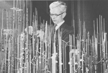
crystallography. Since the first protein structure (myoglobin) was solved by this
technique by John Kendrew and Max Perutz in the late fifties, several
thousand others followed. As can be appreciated from the picture on the right,
which shows John Kendrew with the structural model of myoglobin, at
that time the determination of a structure the size of a protein,
without the aid of a computer, was a formidable task.
It is important to note that in both x-ray crystallography and NMR,
protein structures are not measured directly in the
experiment. Rather, a set of data is collected (a diffraction pattern
or a NMR spectrum), from which a model of the protein structure
is derived. To appreciate the difference between data and structure,
we'll now look at two different structures of the same protein, and
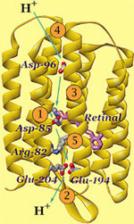
the corresponding x-ray crystallographic data. For this, we will
concentrate on the bacterial light driven proton pump
bacteriorhodopsin. Click
here for more background information on bR.
First download two bR structures from the Protein Data Bank, with PDB entries
1BRR and 1QHJ. Save both PDB files to your local account (see the last
lecture if you forgot how to download from the PDB).
View the structures with rasmol:
rasmol 1BRR.pdb
to focus only on one of the three protein molecules in the file type
(in rasmol):
restrict *a
to see the main features of the structure:
cartoons
color structure
To highlight the dye (the light sensor in the protein interior):
select ret and *a
cpk
Have a close look at the structure, before repeating the procedure for 1QHJ.pdb
in a different window, such that you can compare the two structures.
Question:
By looking at the structures, which of the two structures would you
prefer, in terms of coordinate accuracy?
Remember, so far we only looked at the coordinates, which represent a model
that was optimized against the actually measured data. So, let
us now have a look at the data. In x-ray crystallography, data are
collected by measuring a diffraction pattern that is obtained from
x-rays reflected by a protein crystal. As mentioned in the lecture,
this diffraction pattern itself does not suffice to determine the complete structure
since only the amplitudes of the diffracted waves were collected, not
their phases. In x-ray crystallography, however, there are a number of
tricks available (e.g. isomorphous replacement, molecular replacement)
but we will not go into that in detail here. What is important to
remember is that eventually, an atomic electron density map is obtained.
Question:
Why do primarily the electrons of a molecular sample contribute to the
diffraction of x-rays? answer.
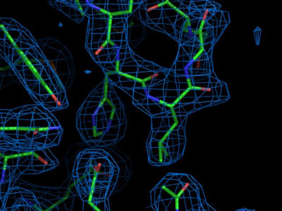
Visit the Uppsala electron density server
to view the electron density map 1BRR. Enter the PDB code (1BRR), and
wait for the summary page to load. Several plots with information on
this structure are available. Feel free to browse around to check the
meaning of the individual plots. At the bottom of the summary, the
electron density viewer can be activated. Select the "Upssala viewer"
instead of the default "Astex viewer" and input that the map should be
centered around residue A83 before clicking "Go". After a while, a
java applet should appear with the electron density and the model
structure visible. Shift the map somewhat to focus on the side-chain
of residue Tyr 83 (by clicking on "center" and then in the atom that
should be centered, until you are in the six-membered aromatic ring).
Do you find the electron density for the aromatic
ring convincing? Now shift the focus to residue A35 (by entering "A35"
in the text field under "center" and then hitting "center"). How is
the fit between the model and the data here? To see the retinal, the
light sensor in the center of the protein, center on A999.
Now repeat the procedure for entry 1QHJ. How is the fit for residue
A35? and for A83? And the retinal (called A300 here)?
Question:
Based on the data and on the model structures, would you say there is
a large impact of the resolution of the data on the accuracy of the structural model?
The highest resolution x-ray crystallographic structures have a
resolution of approx. 0.8A or even somewhat better. To see an example
of such a dataset, look at the density for structure 1G6X, and center
around residue A23. Do you recognize the difference in appearance of
the Tyrosine ring?
Question:
Although the resolution of this structure is rather high, at 0.86A, the
hydrogen atoms (e.g. on the side chain of TYR23) are hardly
visible. Why is this? answer.
NMR
The other main technique for determining protein structures is NMR. In
contrast to x-ray crystallography, no crystals are required for an NMR
experiment. Rather, the structure is determined of the protein in
solution. Therefore, it has the advantage that the protein can be
studied in its native environment. On the other hand, the resolution
of an NMR structure is usually lower and there is a size limitation of
a few hundred amino acids for structure determination using NMR.
It would go beyond the scope of this course to explain the
NMR experiment in detail. We will therefore only briefly touch on the
experimental setup and then focus on the structure building and
refinement step based on the obtained data.
The NMR signal is recorded as a nuclear magnetic resonance spectrum of predominantly the
hydrogen atoms after the sample has been subjected to a (number of)
strong magnetic pulse(s). Mainly hydrogen atoms give rise to the
signal, because of the magnetic spin properties of the hydrogen
nucleus (a proton). The naturally occurring isotopes of the other
elements that are found in proteins, carbon (12C) and
oxygen (16O),
have a zero nuclear magnetic moment. Nitrogen (14N) does
have a non-zero magnetic moment, but can usually not be used in NMR,
for reasons that would go beyond the scope of this course to explain.
These elements, therefore, can only
be utilized in NMR experiments when chemically replaced by a specific
isotope, like 13C or 15N. The most structurally
relevant information is usually obtained from a so called NOESY
experiment (Nuclear Overhauser Enhancement SpectroscopY).
The Nuclear Overhauser Effect or Nuclear Overhauser Enhancement is the
change (enhancement) of the signal intensity from a given nucleus as a
result of exciting or saturating the resonance frequency of another
nucleus. Since this effect is distance-dependent, it can be used to
derive the distance between an interacting pair of protons. In
practice, protons closer than 6A apart can be identified this way.
Now, we will calculate a model of the structure of a small protein,
the B1 domain of protein G,
from the proton-proton distance information obtained from a NOESY
experiment. Download the data file containing the distance information
here. You can have a look at the file
(with the program "more" or "less" or a browser or editor of your
choice) to assure yourself that there are indeed only distance bounds
listed in this file. Additionally, we need an initial guess of the
structure. Since we don't know the structure yet, we have to start from
an unstructured peptide chain, which can be obtained here . Have a look at the structure with:
rasmol proteinG.pdb
Finally, we need something called a
molecular topology, a chemical description of the protein: which atoms
does the molecule contain, which atoms are covalently bonded to each
other, etc. This molecular topology file is available here . Now, in principle, we have all the data
to attempt to build a structure that is in agreement with all
experimentally determined distances. The only thing we still need is
an input file for the
CNS program.
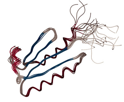
Note that, in contrast to x-ray crystallography, where a
single structure is presented, to reflect the fact that the NMR experiment probes
an ensemble of protein molecules in solution, an NMR structure is
usually represented by an ensemble of structures, that all fulfill the
NMR data. Start CNS with
tcsh
source /usr/global/cns/cns_solve_env
cns < anneal.inp
10 structures of the B1 domain of protein G will now be calculated by
simulated annealing. This is a computationally intensive calculation,
as the structure is slowly, dynamically transformed from the extended
starting conformation to the real structure, by a slow-cooling
simulation, also called simulated annealing. As the calculation is
running, we can have a look at how exactly such a calculation proceeds,
and how the final structure is generated from the starting
guess. Download this file, open another shell, and
open the just downloaded file in pymol:
/usr/global/whatif/pymol/pymol sa.pdb
on the white bar, in the top pymol window, type:
show cartoon
and then press the "play" button at the bottom right of the main pymol
window, to see an animation of the simulated annealing structure
calculation procedure. If the movie plays too fast, on the menu, under
movie -> speed, choose a different speed.
When the CNS structure calculation has finished, switch back to that
window and type:
cat anneala_*.pdb > anneal.pdb
to combine all ten generated structures into one file. View the result
with:
rasmol anneal.pdb
Question:
Which parts of the structure are well-defined, and which parts show
more ambiguity?
There is also a x-ray structure available of the B1 domain of protein
G, available under the PDB code 1PGB. Download it from the Protein Data Bank and compare it to
the just calculated NMR structure.
Question:
What are the main differences between the NMR and x-ray structures of
the B1 domain of protein G? hint