Molecular Dynamics simulations of proteins

Analysis of a gromacs simulation

The simulation is running now (or finished) and we can start analysing

the results. Let us first see which kind of files have been written by

the simulation (mdrun):

ls -lrt

We see the following files:

traj.xtc - the trajectory to be used for analyses
traj.trr - the trajectory to be used for a restart in case of a crash
ener.edr - energies
md.log - a LOG file of mdrun
md.gro - the final coordinates of the simulation

The first analysis step during or after a simulation is usually a

visual inspection of the trajectory. For this we will use the gromacs

trajectory viewer ngmx. Other possibilities would be VMD , Pymol, or gOpenmol.

ngmx -s md.tpr -f traj.xtc

Select a group of your interest ("system" might be good for a start),

and then, under "Display", click "Animate". Now a animation player

button appears near the bottom of the screen, which can be used to

view the trajectory. If you wish to filter different simulated

components, choose a different group under "Display" and "Filter".

We can see that the protein and its surroundings undergo thermal

fluctuations, but overall, the protein structure is rather stable, as

would be expected on such timescales.

A more versatile visualisation is provided by pymol. First, we have to extract

the protein coordinates and write to PDB format:

trjconv -s md.tpr -f traj.xtc -o traj.pdb -dt 1.

Now, select group 1 (Protein). And view with pymol:

/usr/global/whatif/pymol/pymol traj.pdb

On the pymol prompt, type:

dss

followed by

show cartoon

Play the animation by pressing the play button.

For a more quantitative analysis

on the protein fluctuations, we can view how fast and how far the

protein deviates from the starting (experimental) structure:

g_rms -s md.tpr -f traj.xtc

When prompted for groups to be analysed, type "1 1 1". g_rms has

written a file called "rmsd.xvg", which can be viewed with:

xmgrace rmsd.xvg

We see the Root Mean Square Deviation (rmsd) from the starting

structure, averaged over all protein atoms, as a function of time. The

deviation of 0.1 nm is within the expected range for a protein like

the B1 domain at a temperature of 300K at such timescales. If we now

wish to see if the fluctuations are equally distributed over the

protein, or if some residues are more flexible than others, we can

type:

g_rmsf -s md.tpr -f traj.xtc -oq

Select group "3" (C-alpha). The result can be viewed with:

xmgrace rmsf.xvg

We can see that mainly two regions in the protein show a large

flexibility: around residue 11 and residue 48. To see where these

residues are located in the protein, type:

rasmol bfac.pdb

Under "Colours", select "Temperature". The protein backbone is now

shown with the flexibility encoded in the colour. The red (orange,

green) regions are relatively flexible and the blue regions are

relatively rigid. It can be seen that the alpha-helix and beta-sheet

are relatively stable, whereas the loops are more flexible.

Repeat the same rasmol command for the x-ray structure (1PGB.pdb).

Question: How do the flexibilities in the simulation compare to the temperature factors in the crystallographic structure?

(note that the correspondence cannot be expected to be 100%, as the protein flexibility in different in the crystal than in solution (as in the simulation). Additionally, not only flexibility is encoded in the crystallographic B-factor, but also experimental error or model inaccuracy)

The simulation not only yields information on the structural

properties of the simulation, but also on the energetics. With the

program

g_energy the energies written by mdrun can be analysed:

g_energy -f ener.edr

Select "Potential" and end your selection by pressing enter twice, View the result with:

xmgrace energy.xvg

As can be seen, the total potential energy initially rises rapidly after

which it relaxes again.

Question: can you think of an explanation for

this behaviour?

Please repeat the energy analysis for a number of different energy

terms to obtain an impression of their behaviour.

We continue with a number of more specific analysis, the first of

which is an analysis of the secondary structure (alpha-helix,

beta-sheet) of the protein during the simulation.

First, we need to tell gromacs where the DSSP program for secondary structure

calculations can be found:

export DSSP=/usr/global/whatif/dssp/dssp

(or, if you get a message "export: Command not found.", you're perhaps using a

(t)csh in which case the command should be:)

setenv DSSP /usr/global/whatif/dssp/dssp

Now, perform the actual analysis with:

do_dssp -s md.tpr -f traj.xtc

select group "1" (protein), and convert the output to PostScript with:

xpm2ps -f ss.xpm

and view the result with:

gv plot.eps

if "gv" is not installed on your computer, try "xpsview", "ghostview"

or "gs". As can be seen, the secondary structure is rather stable

during the simulation, which is an important validation check of the

simulation procedure (and force-field) used. The next thing to analyse

is the change in the overall size (or gyration radius) of the protein:

g_gyrate -s md.tpr -f traj.xtc

(again, select group "1" for the protein)

xmgrace gyrate.xvg

The analysis shows that the gyration radius fluctuates around a stable

value and does not show any significant drift. Another important check

concerns the behaviour of the protein surface:

g_sas -s md.tpr -f traj.xtc

(again, select group "1" for the protein)

xmgrace -nxy area.xvg

We now see three curves together: black for the hydrophobic accessible

surface, red for the hydrophilic accessible surface, and green for the

total accessible surface.

Question: Is the total

(solvent-accessible) surface constant? Are any hydrophobic groups

exposed during the simulation?

OPTIONAL

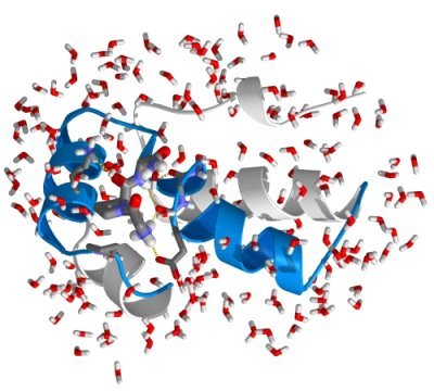
You've probably noticed that in the simulation about only ten percent of the

system that was simulated consisted of protein, the rest was water. As we are

mainly interested in the protein's motions and not so much in the surrounding

water, one could ask if we couldn't forget about the water and rather simulate

the protein. That way, we could reach ten times longer simulations with the

same computational effort!

Question: Why do you think that it is

important to include explicit solvent in the simulation of a protein?

To check if your assumption is correct, repeat the simulation of protein G,

this time without solvent (to observe the effect more clearly, increase the

length of the simulation by changing "nsteps" in the file "md.mdp" by e.g. a

factor of ten).

Question: What are the main differences to the

protein's structure and dynamics as compared to the solvent simulation?

(Hint: use programs like g_rms and g_gyrate to analyse both simulations).